Final exam（60%）
期末考试@W15~16期末周
考试形式：开卷（120min）
*考试内容：
1.MCQ: 54 Marks
2.Filling blanks: 24 Marks
3.Computation: 14 Marks
4.Essay Question: 8 Marks

Lectures

周数	主题	内容1	教科书章节	内容2	考试
1	概述		Ch 1	Python基础
2	数据特征	机器学习概述	Ch 2
3		降维	Ch 8
4		数据观测练习		作业指导&反馈
5	监督学习	数据分类/模型训练	Ch 3~4		数据观测
6		监督学习I	Ch 5
7		这周不知道干什么
8		监督学习II	Ch 6~7
9		数据分类练习		作业指导&反馈
10	无监督学习	无监督学习	Ch 9		分类
11		聚类练习
12		AI应用		作业指导&反馈	聚类
13	复习总结

Lecture 3:

This lecture mainly focused on the Dimensionality Reduction and two ways to achieve it. They are Principal Component Analysis(PCA) and Locally Linear Embedding(LLE).

Dimensionality Reduction（降维）

The drawback of the data with high dimensions:

High computational complexity
May contain many irrelevant or redundant features.
Difficulty in visualization
With high risk of getting an overfitting model

The approaches for Dimensionality Reduction:

Projection:

Data is not spread out uniformly across all dimensions. All the data lies within (or close to) a much lower-dimensional subspace of the high-dimensional space.

Principal Component Analysis

The PCA is one of the methods for dimensions reduction. For example, assume that we have to describe an object with two features. However, our model is only capable of processing just one of them. We then have to reduce the dimensions of the data set. In a gesture to represent both of the feature, we have to find a new coordinate to measure these data. And that is what pac is doing. Since there are two features in this case, We aim to disperse the data as much as possible in the new coordinate system, so we need to find a coordinate system that makes the data more scattered. And that is the picture above shows us.

The concept below is Comparatively challenging, so I would show my understandings in both Chinese and English.

新坐标系的寻找可以被简单的看成是原坐标系的拉伸和旋转。由此我们可以得到方程（方程式的推导有些复杂，并且学校并不考察相关步骤，这里就不做拓展）。其中，这里面的c1和c1的传置，就是新坐标系的“横纵“坐标，也就是上图显示的c1和c2的位置。根据线性代数的推导（感兴趣的话可以自己试一试），我们可以知道协方差矩阵的特征向量就是c1。c1的传置就是c1T。S就是角度旋转的平方。所以要求新的坐标系，那么就是需要求出协方差矩阵的特征向量。

The search for the new coordinate system can be simplified as the stretching and rotation of the original coordinate system. Consequently, we can derive the following equation (the derivation of the equation is somewhat complex, and as it is not examined in school, we won’t delve into it here). Here, c1 and its transpose in the equation represent the ‘horizontal’ and ‘vertical’ coordinates of the new coordinate system, akin to the positions of c1 and c2 illustrated in the above diagram. Through linear algebra derivations (which you can explore on your own if interested), we understand that the eigenvectors of the covariance matrix are precisely c1. The transpose of c1 is denoted as c1T. S denotes the square of the angle of rotation. Hence, to determine the new coordinate system, we need to find the eigenvectors of the covariance matrix.

下面是对整个定理的证明，核心思想是用拉格朗日定理来将新的坐标轴在以1为模长的范围内的最大值。简单了解即可，最重要的是会做计算题和选择题。

The picture above is the proof for the entire theorem. The central idea is to use Lagrange’s theorem to maximize the new coordinate axes within a range of length 1. A basic understanding is sufficient; the most crucial aspect is the ability to solve computational and multiple-choice questions.

Exercises:

Given a dataset that consists of the following points below:
A=(2, 3), B=(5, 5), C=(6, 6), D=(8,9)
1. Calculate the covariance matrix for the dataset.
2. Calculate the eigenvalues and eigenvectors of the covariance matrix.

The calculation provided by the professor is given below:

I strongly recommend you to conduct the calculation on your own to familiar with the details.(Don’t be so cocky. Practice makes perfect). Here the std is deliberately made to 2.5 to simply the calculation. And the data normalization is mainly using z-score normalization.

Singular Value Decomposition (SVD)

SVD揭示了这样的一个事实:对于任意的矩阵A,我们总能找到一组单位正交基, 使得A对其进行变换之后, 得到的向量组仍然是正交的.

SVD其实在我上面讲解公式的时候已经用到了类似的思想了，也就是将坐标系进行拉伸和旋转。下面是学校提供的公式：

SVD reveals the following fact: for any matrix AA, it is always possible to find a set of unitary orthogonal bases such that, after transforming AA with respect to these bases, the resulting vector set remains orthogonal.

The concept used in the explanation of formulas above is akin to SVD, involving the stretching and rotating of coordinate systems. The following are the provided formulas from the school:(To be continued)

Lecture 4：

Bayes’ Rule：

贝叶斯定理是一个比较简单的逻辑概念，本身的运算并不复杂。如果后续学校需要跟进知识的广度，这里会继续展开。

下面是CW1过Demonstration的战术总结：

按照学校matlab的示例代码转化成python，自己搞一遍，然后给老师看。然后进行下面的论述：

首先我们要分析一下数据，针对于学校给出的一些特征，我们需要对他们进行相关性的判断。比较常见的方法是热力图来画出图像来分析特征相对于目标特征的一些相关性。（里面是统计学的知识，这里不做展开，你只需要知道这里面是相关性系数就行了，范围在-1到1之间，图像里面颜色越深代表相关性越强，一条1.0的线代表是和自己作比较的分割线。）

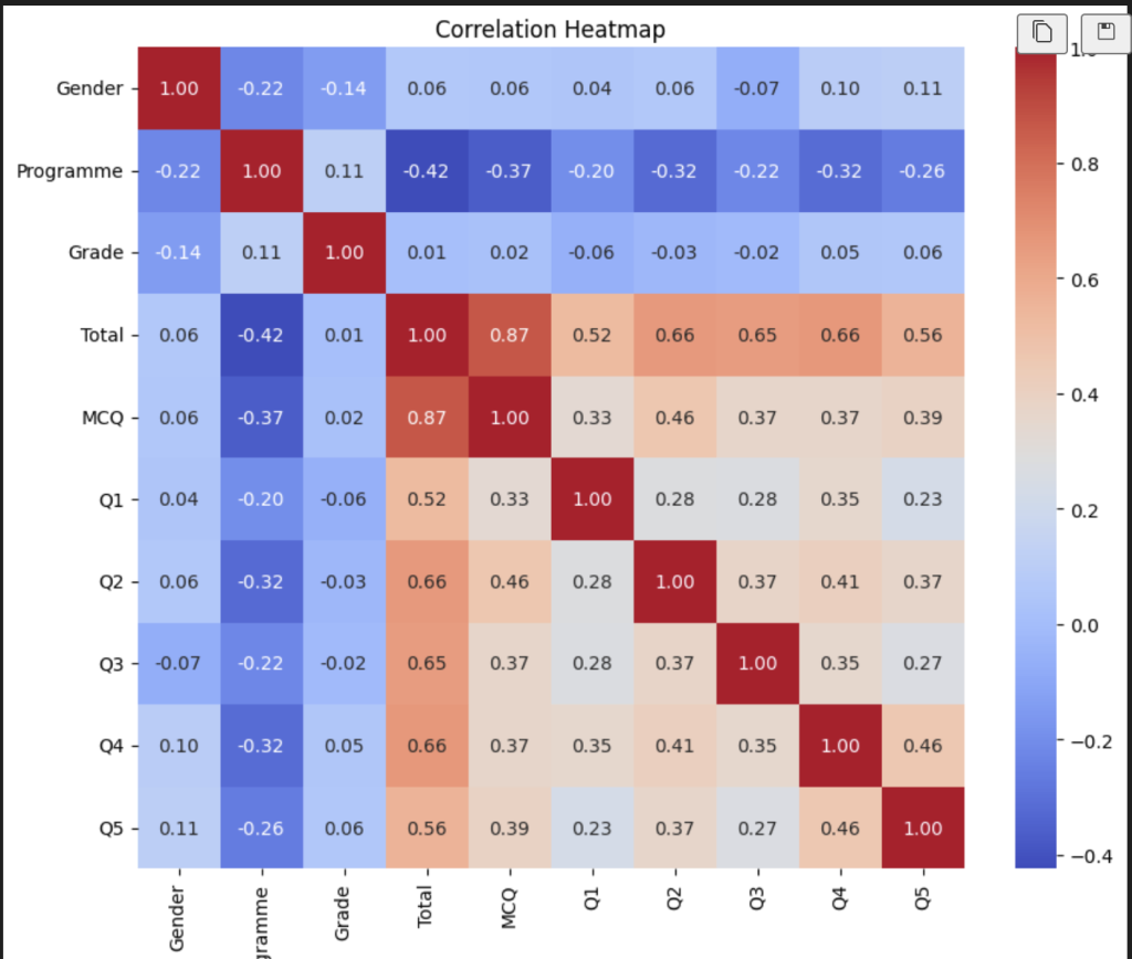
由此我们可以注意到：Total，MCQ，Q2，Q4都与programme有着较好的相关性。所以我们可以尝试只对这些变量作pca或者tsne降维处理。结果如下（tsne）：

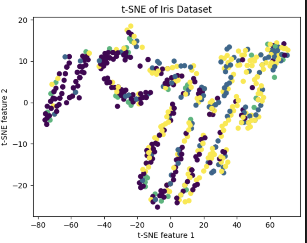
发现其实效果并不是特别的好，于是我们大力出奇迹。把所有的东西都放在pca当中（当然这里面的数据要除去index还有programme自身）。效果如下：

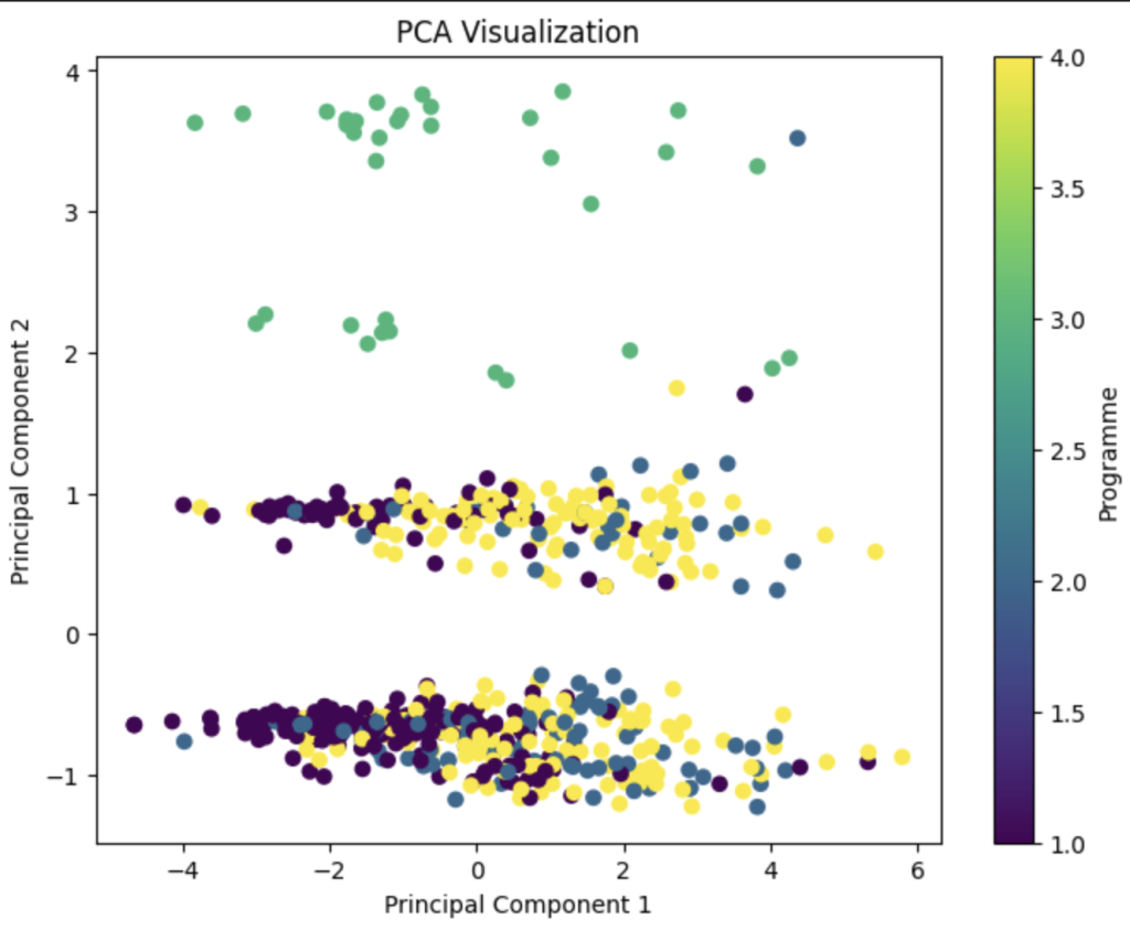
这就是一个效果比较好的图像了。因为我们可以用肉眼观测到差异。programme3显然和其他的programme有着差异。所以我们就对分析好的数据进行了一个比较令人满意的降维了。（当然这里面处理数据的方法有很多，肯定不止我这一种，喜欢钻研的话可以自己用一些其他的特征来操作一下）参考代码如下：

import pandas as pd
import seaborn as sns
import matplotlib.pyplot as plt

data = pd.read_excel(“CW_Data.xlsx”)
correlation_matrix = data.drop(columns=[‘Index’]).corr()
#绘制热力图
plt.figure(figsize=(10, 8))
sns.heatmap(correlation_matrix, annot=True, cmap=’coolwarm’, fmt=”.2f”, annot_kws={“size”: 10})
plt.title(‘Correlation Heatmap’)
plt.show()


#t-sne降维
from sklearn.manifold import TSNE
X = data[['Grade','Total','MCQ']]
y = data['Programme']
 
# 应用t-SNE
tsne = TSNE(n_components=2, random_state=0)
X_tsne = tsne.fit_transform(X)
 
# 可视化结果
plt.scatter(X_tsne[:, 0], X_tsne[:, 1], c=y)
plt.xlabel('t-SNE feature 1')
plt.ylabel('t-SNE feature 2')
plt.title('t-SNE of Iris Dataset')
plt.show()

# 提取特征和目标变量
import pandas as pd
data = pd.read_excel("CW_Data.xlsx")
X = data[['Total','Gender','MCQ','Q4','Q3','Q2','Q1','Q5','Grade']]
y = data['Programme']
data
print(X)


# 最后的pca
# 标准化数据。（归一化）
scaler = StandardScaler()
X_scaled = scaler.fit_transform(X)

# 使用PCA进行降维
pca = PCA(n_components=2)
X_pca = pca.fit_transform(X_scaled)

# 可视化降维结果
plt.figure(figsize=(8, 6))
plt.scatter(X_pca[:, 0], X_pca[:, 1], c=y, cmap='viridis')
plt.xlabel('Principal Component 1')
plt.ylabel('Principal Component 2')
plt.title('PCA Visualization')
plt.colorbar(label='Programme')
plt.show()

Eachone

INT 104

INT104_240310时间线与课程信息

概述信息

教师联系方式

Module Leader

Teaching Staff